import numpy as np
import scipy.stats as st
import matplotlib.pyplot as plt

B = st.binom(1000, 0.001) # random variable

k = np.arange(1001)
B.pmf(k) # density function, AKA probability mass function

array([0.36769542, 0.36806349, 0.18403174, ..., 0.        , 0.        ,
       0.        ])

plt.scatter(k, B.pmf(k));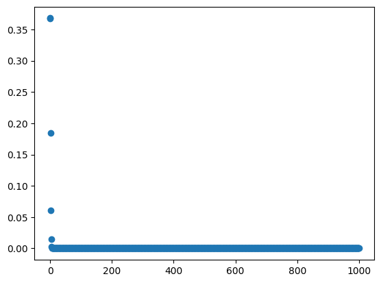

np.sum(B.pmf(np.arange(100, 1001))) # P[X >= 100]

2.6181505053540243e-161

np.sum(B.pmf(np.arange(51))) # P[X <= 50]

1.0

Some examples from https://roualdes.us/lecturenotes/binomial

# 1.
B1 = st.binom(10, 0.95)
B1.pmf(10) # a
B1.pmf(8)  # b

0.07463479852001967

# 2.
B2 = st.binom(50, 0.1)
np.sum(B2.pmf(np.arange(3, 51)))

0.8882712436536537

# 3.
B3 = st.binom(10, 0.7)
np.sum(B3.pmf(np.arange(8, 11)))

0.3827827864000003