Central Limit Theorem

import numpy as np
import matplotlib.pyplot as plt
import scipy.stats as spicy

rng = np.random.default_rng()
N = 1001
R = 1

x = rng.exponential(5.3, size = (R, N))
ndx = np.arange(1, N + 1)
cm = np.cumsum(x, axis = 1) / ndx

plt.plot(ndx, cm.T);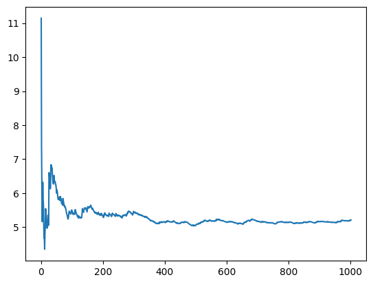

plt.hist(x[0], histtype = "step", density = True, bins = 17);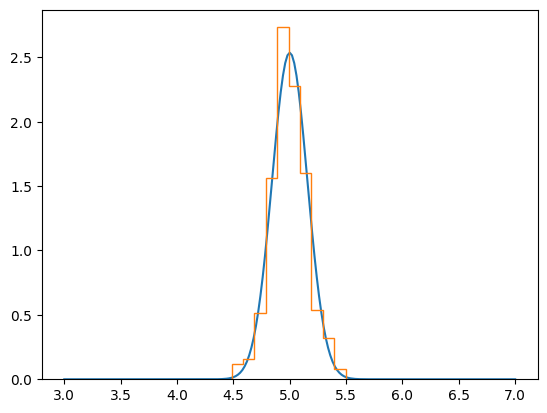

plt.hist(cm[:, 900], histtype = "step", density = True, bins = 17);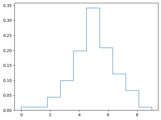

xbar = np.mean(x[0])
z = spicy.norm().ppf(0.975) # 95%
xbar - z * 5.3 / np.sqrt(np.size(x[0])), xbar + z * 5.3 / np.sqrt(np.size(x[0]))

(4.883685307715739, 5.54033979675485)

Assume the random variables \(X_1, \ldots, X_N\) are independent and all come from the same distribution, let’s call this distribution \(F\). So long as \(\mathbb{V}[X] = \sigma^2 < \infty\), then

\[\frac{\bar{X} - \mu}{\sigma / \sqrt{N}} \quad \dot{\sim} \quad \text{Normal}(0, 1)\]

where \(\mathbb{E}[X] = \mu\).

Note that we don’t care what \(F\) looks like, symmetric, skewed, multi-modal. So long as \(F\) has finite variance, then the mean of random variables from \(F\) is itself a random variable. The Central Limit Theorem says that the approximate shape of \(\bar{X}\), after centering and scaling it appropriately, is a standard Normal distribution (located/centered at \(0\) and scaled to a variance of \(1\)).

Because of the Central Limit Theorem, we can theoretically calculate probabilities that the random variable \(\frac{\bar{X} - \mu}{\sigma/\sqrt{N}}\) is between two numbers \(-z, z\). In fact, we can find a number \(z\) such that the probability is equal to say 0.95,

\[\mathbb{P}\left[-z \leq \frac{\bar{X} - \mu}{\sigma/\sqrt{N}} \leq z\right] = 0.95\]

spicy.norm().ppf(0.975) # for 95%, z =

1.959963984540054

Re-working the inequality inside the probability statement gives us a way to bound with a specified probability the expectation, \(\mu = \mathbb{E}[X]\).

\[\mathbb{P}\left[\bar{X} - z \sigma / \sqrt{N} \leq \mu \leq \bar{X} + z \sigma / \sqrt{N} \right]\]

Hence, a reasonable starting point to bound with high probability the expectation \(\mu = \mathbb{E}[X]\) is

\[\bar{X} \pm z \sigma / \sqrt{N}\]

The problem is that this formula requires knowledge of the standard deviation \(\sigma = \sqrt{\mathbb{V}[X]}\). Since it is extremely unlikely that we have this, we’ll have to estimate it, too. We’ll have to estimate both the expectation with \(\bar{X}\) and the standard deviation. We next to turn confidence intervals under the t-distribution.

Other Formats