import numpy as np
import matplotlib.pyplot as plt
import scipy.stats as spicy

In the Central Limit Theorem notes, we learned a framework for which we can bound an expectation. However, we don’t want to rely on knowledge of the standard deviation. When you have to estimate the standard deviation, in order to bound with a confidence interval, the expectation, we must use the formula

\[\bar{X} \pm t_{N-1} s / \sqrt{N}\]

where \(t_{N-1}\) is found from the t-distribution. If \(N = 10\), then we could use the following code to find \(t_{N-1}\)

spicy.t(df = 10 - 1).ppf(0.975) # for 95% confidence interval

2.262157162854099

rng = np.random.default_rng()

N = 1000
R = 10_000
b = np.zeros(R)
n = 11
p = 0.75
E = n * p
for r in range(R):
    x = rng.binomial(n, p, size = N)
    xbar = np.mean(x)
    t = spicy.t(df = N - 1).ppf(0.95) # t-distribution to acccount
    # for estimating mean and standard deviation (two things)
    s = np.std(x)
    lb = xbar - t * s / np.sqrt(N)
    ub = xbar + t * s / np.sqrt(N)
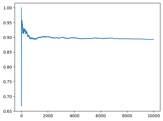
    b[r] = lb <= E <=  ub # Bernoulli

np.mean(b)

0.8932

rdx = np.arange(1, R+1)
cm = np.cumsum(b) / rdx
plt.plot(rdx, cm);