linear_in_what – lectures

import matplotlib.pyplot as plt
import numpy as np
import pandas as pd
import statsmodels.formula.api as smf

# same link as for finches -> carnivora
df = pd.read_csv("https://raw.githubusercontent.com/roualdes/data/refs/heads/master/carnivora.csv")

df.head()

	Order	SuperFamily	Family	Genus	Species	FW	SW	FB	SB	LS	GL	BW	WA	AI	LY	AM	IB
0	Carnivora	Caniformia	Canidae	Canis	Canis lupus	31.1	33.1	130.0	132.3	5.5	63.0	425.0	35.0	NaN	177.0	913	12
1	Carnivora	Caniformia	Canidae	Canis	Canis latrans	9.7	10.6	84.5	88.3	6.2	61.5	225.0	98.0	NaN	NaN	365	12
2	Carnivora	Caniformia	Canidae	Canis	Canis adustus	10.6	11.3	53.5	51.8	4.3	63.3	NaN	NaN	NaN	127.0	NaN	NaN
3	Carnivora	Caniformia	Canidae	Canis	Canis mesomelas	7.2	7.7	52.0	56.8	3.8	60.0	NaN	61.0	270.0	NaN	392	NaN
4	Carnivora	Caniformia	Canidae	Lycaon	Lycaon pictus	22.2	22.0	128.0	129.0	8.8	70.5	365.0	77.0	390.0	132.0	t 132	13

plt.scatter(df["SW"], df["SB"])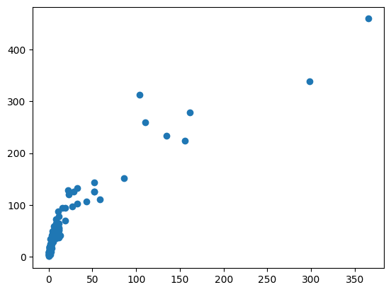

model = smf.ols("SB ~ SW + I(SW* SW)", data = df)
fit = model.fit()

fit.summary()

OLS Regression Results
Dep. Variable:	SB	R-squared:	0.915
Model:	OLS	Adj. R-squared:	0.913
Method:	Least Squares	F-statistic:	585.6
Date:	Thu, 20 Nov 2025	Prob (F-statistic):	4.93e-59
Time:	08:58:06	Log-Likelihood:	-503.95
No. Observations:	112	AIC:	1014.
Df Residuals:	109	BIC:	1022.
Df Model:	2
Covariance Type:	nonrobust

	coef	std err	t	P>\|t\|	[0.025	0.975]
Intercept	21.3680	2.423	8.818	0.000	16.565	26.171
SW	2.2409	0.110	20.355	0.000	2.023	2.459
I(SW * SW)	-0.0032	0.000	-8.822	0.000	-0.004	-0.003

Omnibus:	26.840	Durbin-Watson:	1.275
Prob(Omnibus):	0.000	Jarque-Bera (JB):	70.392
Skew:	0.848	Prob(JB):	5.18e-16
Kurtosis:	6.494	Cond. No.	1.83e+04

Notes:
[1] Standard Errors assume that the covariance matrix of the errors is correctly specified.
[2] The condition number is large, 1.83e+04. This might indicate that there are
strong multicollinearity or other numerical problems.

mn, mx = np.min(df["SW"]), np.max(df["SW"])
ndf = pd.DataFrame.from_dict({
    "SW": np.linspace(mn, mx, 101)
})
ndf["yhat"] = fit.predict(ndf)
plt.scatter(df["SW"], df["SB"])
plt.plot(ndf["SW"], ndf["yhat"], color = "black")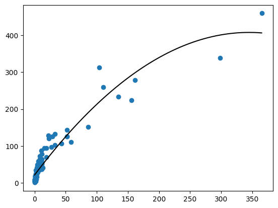

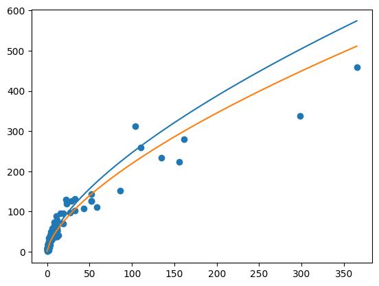
plt.scatter(np.log10(df["SW"]), np.log10(df["SB"]))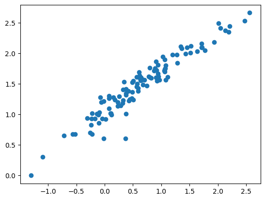

model = smf.ols("np.log10(SB) ~ np.log10(SW)", data = df)
fit = model.fit()

yhat = fit.predict(df)
plt.scatter(df["SW"], df["SB"])
plt.plot(df["SW"], yhat)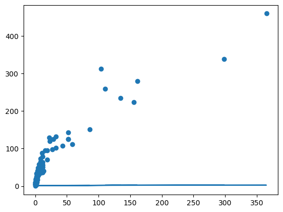

mn, mx = np.min(df["SW"]), np.max(df["SW"])
ndf = pd.DataFrame.from_dict({
    "SW": np.linspace(mn, mx, 101)
})
ndf["yhat"] = fit.predict(ndf)
plt.scatter(df["SW"], df["SB"])
plt.plot(ndf["SW"], 10 ** ndf["yhat"], color = "black")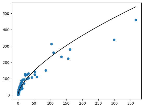

# instantiate and fit model here: log10 both x, y, and 
# unique "intercepts" by SuperFamily

mn, mx = np.min(df["SW"]), np.max(df["SW"])
x = np.linspace(mn, mx, 101)
ndf = pd.DataFrame.from_dict({
    "SuperFamily": np.repeat(["Caniformia", "Feliformia"], 101),
    "SW": np.tile(x, 2)
})
ndf["yhat"] = fit.predict(ndf)


# make plot here: one line for each SuperFamily

Other Formats