Linear Regression

import matplotlib.pyplot as plt
import numpy as np
import pandas as pd
import statsmodels.api as sm
import statsmodels.formula.api as smf
import patsy as pt

hospital = pd.read_csv("https://raw.githubusercontent.com/roualdes/data/refs/heads/master/hospital.csv")

plt.scatter(hospital["stay"], hospital["infection_risk"])
plt.xlabel("Stay (days)")
plt.ylabel("Infection risk");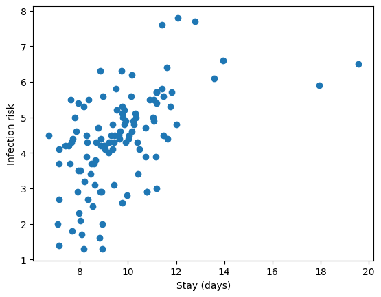

fit = smf.ols("infection_risk ~ nurses * stay", data = hospital).fit()
fit.summary()

OLS Regression Results
Dep. Variable:	infection_risk	R-squared:	0.349
Model:	OLS	Adj. R-squared:	0.331
Method:	Least Squares	F-statistic:	19.48
Date:	Tue, 02 Dec 2025	Prob (F-statistic):	3.48e-10
Time:	22:24:29	Log-Likelihood:	-168.73
No. Observations:	113	AIC:	345.5
Df Residuals:	109	BIC:	356.4
Df Model:	3
Covariance Type:	nonrobust

	coef	std err	t	P>\|t\|	[0.025	0.975]
Intercept	-0.3488	0.989	-0.353	0.725	-2.308	1.611
nurses	0.0089	0.004	1.993	0.049	5.08e-05	0.018
stay	0.4498	0.106	4.253	0.000	0.240	0.659
nurses:stay	-0.0007	0.000	-1.499	0.137	-0.002	0.000

Omnibus:	0.593	Durbin-Watson:	1.878
Prob(Omnibus):	0.744	Jarque-Bera (JB):	0.716
Skew:	0.153	Prob(JB):	0.699
Kurtosis:	2.758	Cond. No.	2.27e+04

Notes:
[1] Standard Errors assume that the covariance matrix of the errors is correctly specified.
[2] The condition number is large, 2.27e+04. This might indicate that there are
strong multicollinearity or other numerical problems.

ndf = pd.DataFrame.from_dict({"stay": [20, 20], "nurses": [100, 101]})
np.diff(fit.predict(ndf))

array([-0.00447639])

For each extra nurse, when stay is equal to 20, we expect infection risk to decrease by 0.004.

ndf = pd.DataFrame.from_dict({"stay": [10, 10], "nurses": [100, 101]})
np.diff(fit.predict(ndf))

array([0.00221305])

For each extra nurse, when stay is equal to 10, we expect infection risk to increase by 0.002.

Logistic Regression

# change hospital -> possum
possum = pd.read_csv("https://raw.githubusercontent.com/roualdes/data/refs/heads/master/possum.csv")

possum["vic"] = (possum["pop"].astype("string") == "vic").astype(np.float64)

rng = np.random.default_rng()
N = np.shape(possum)[0]
plt.scatter(possum["tailL"] + rng.uniform(size = N) * 0.25, possum["vic"], 
            alpha = 0.25);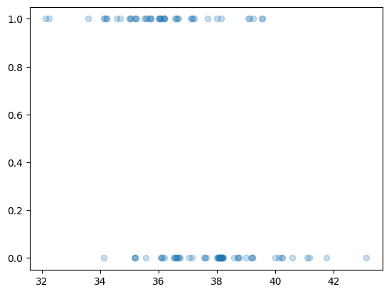

fit = smf.glm("vic ~ age * tailL", data = possum, 
              family = sm.families.Binomial()).fit()

fit.summary()

Generalized Linear Model Regression Results
Dep. Variable:	vic	No. Observations:	102
Model:	GLM	Df Residuals:	98
Model Family:	Binomial	Df Model:	3
Link Function:	Logit	Scale:	1.0000
Method:	IRLS	Log-Likelihood:	-53.011
Date:	Tue, 02 Dec 2025	Deviance:	106.02
Time:	22:24:29	Pearson chi2:	113.
No. Iterations:	5	Pseudo R-squ. (CS):	0.2796
Covariance Type:	nonrobust

	coef	std err	z	P>\|z\|	[0.025	0.975]
Intercept	49.3407	15.472	3.189	0.001	19.016	79.665
age	-5.5348	3.032	-1.825	0.068	-11.478	0.409
tailL	-1.3680	0.422	-3.239	0.001	-2.196	-0.540
age:tailL	0.1554	0.082	1.887	0.059	-0.006	0.317

x = np.linspace(32, 44, 101)
m = np.mean(possum["age"])
ndf = pd.DataFrame.from_dict({"tailL": x, "age": np.full(101, m)})
yhat = fit.predict(ndf)

plt.scatter(possum["tailL"] + rng.uniform(size = N) * 0.25, possum["vic"], 
            alpha = 0.25);
plt.plot(x, yhat);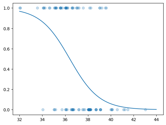

ndf = pd.DataFrame.from_dict({"tailL": [37, 38], "age": [m, m]})
np.diff(fit.predict(ndf))

array([-0.16145695])

Other Formats

Logistic Regression