multiple_linear_regression

import matplotlib.pyplot as plt
import numpy as np
import pandas as pd
import statsmodels.api as sm # pip install -U statsmodels patsy 
import statsmodels.formula.api as smf
import patsy as pt

df = pd.read_csv("https://raw.githubusercontent.com/roualdes/data/refs/heads/master/finches.csv")

df.head()

	island	winglength	taillength	beakwidth	beakheight	lowerbeaklength	upperbeaklength	tarsuslength	middletoelength
0	santacruz	63.5	40.0	9.0	11.0	9.0	16.0	20.0	18.5
1	santacruz	69.5	41.0	9.0	12.0	8.5	16.0	21.2	19.5
2	santacruz	70.0	44.0	9.2	12.0	8.5	16.0	21.0	18.6
3	santacruz	70.0	43.5	9.2	11.2	8.5	16.2	20.5	19.0
4	santacruz	70.5	42.0	9.5	12.0	8.5	16.5	22.0	19.2

plt.scatter(df["beakwidth"], df["winglength"]);

y, X = pt.dmatrices("winglength ~ island + beakwidth", data = df) # design matricess
X[20:40]

array([[ 1. ,  1. ,  0. , 10. ],
       [ 1. ,  1. ,  0. , 10.2],
       [ 1. ,  1. ,  0. , 11. ],
       [ 1. ,  1. ,  0. , 10.5],
       [ 1. ,  1. ,  0. , 11. ],
       [ 1. ,  1. ,  0. , 10. ],
       [ 1. ,  1. ,  0. , 12. ],
       [ 1. ,  1. ,  0. , 11. ],
       [ 1. ,  1. ,  0. , 11. ],
       [ 1. ,  1. ,  0. ,  9.5],
       [ 1. ,  1. ,  0. , 11. ],
       [ 1. ,  1. ,  0. , 10.2],
       [ 1. ,  1. ,  0. , 12. ],
       [ 1. ,  1. ,  0. , 11.5],
       [ 1. ,  1. ,  0. , 11.5],
       [ 1. ,  1. ,  0. , 11.2],
       [ 1. ,  1. ,  0. , 12. ],
       [ 1. ,  1. ,  0. , 12.2],
       [ 1. ,  1. ,  0. , 12.5],
       [ 1. ,  1. ,  0. , 11.5]])

model = smf.ols("winglength ~ island * beakwidth", data = df)
fit = model.fit()

fit.summary()

OLS Regression Results
Dep. Variable:	winglength	R-squared:	0.771
Model:	OLS	Adj. R-squared:	0.753
Method:	Least Squares	F-statistic:	41.82
Date:	Thu, 13 Nov 2025	Prob (F-statistic):	1.30e-18
Time:	13:49:11	Log-Likelihood:	-140.68
No. Observations:	68	AIC:	293.4
Df Residuals:	62	BIC:	306.7
Df Model:	5
Covariance Type:	nonrobust

	coef	std err	t	P>\|t\|	[0.025	0.975]
Intercept	49.0160	2.211	22.172	0.000	44.597	53.435
island[T.sancristobal]	-0.0065	3.812	-0.002	0.999	-7.627	7.615
island[T.santacruz]	-7.6337	4.943	-1.544	0.128	-17.514	2.247
beakwidth	2.3143	0.226	10.229	0.000	1.862	2.767
island[T.sancristobal]:beakwidth	-0.1547	0.367	-0.421	0.675	-0.889	0.579
island[T.santacruz]:beakwidth	0.5926	0.484	1.226	0.225	-0.374	1.559

Omnibus:	7.089	Durbin-Watson:	2.007
Prob(Omnibus):	0.029	Jarque-Bera (JB):	3.781
Skew:	-0.362	Prob(JB):	0.151
Kurtosis:	2.100	Cond. No.	256.

Notes:
[1] Standard Errors assume that the covariance matrix of the errors is correctly specified.

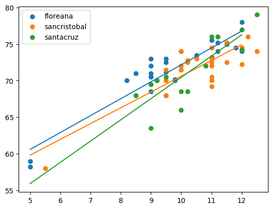
for name, gdf in df.groupby(["island"]):
    plt.scatter(gdf["beakwidth"], gdf["winglength"], label = name[0]);
plt.legend();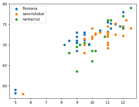

xnew = np.array([5, 12])
ndf = pd.DataFrame.from_dict({"beakwidth": xnew, 
                              "island": ["floreana", "floreana"]})
ndf["yhat"] = fit.predict(ndf)
ndf

	beakwidth	island	yhat
0	5	floreana	60.587695
1	12	floreana	76.788024

for name, gdf in df.groupby(["island"]):
    plt.scatter(gdf["beakwidth"], gdf["winglength"], label = name[0]);
    xnew = np.array([5, 12])
    ndf = pd.DataFrame.from_dict({"beakwidth": xnew, 
                              "island": [name[0], name[0]]})
    ndf["yhat"] = fit.predict(ndf)
    plt.plot(xnew, ndf["yhat"])
plt.legend();

Other Formats