MATH 315 Practice Exam 02

  1. Describe the Central Limit Theorem and also include why it’s appropriate to use a symmetric confidence interval.

  2. Consider the variable LS (litter size) from the carnivora dataset. The output of a t-test is below. Answer the following question based on this output.

    carnivora <- read.csv("https://raw.githubusercontent.com/roualdes/data/refs/heads/master/carnivora.csv")
    t.test(carnivora$LS, mu = 2, conf.level = 0.9)
    
     One Sample t-test
    
    data:  carnivora$LS
    t = 9.87, df = 109, p-value < 2.2e-16
    alternative hypothesis: true mean is not equal to 2
    90 percent confidence interval:
     3.024773 3.438863
    sample estimates:
    mean of x 
     3.231818 
    1. How many observations were measured / what is the sample size?

    2. Interpret, in context of these data, the confidence interval.

    3. Did this confidence interval capture the true population parameter it is targeting?

    4. If we had instead more observations in the sample, would the confidence interval be narrower or wider? Explain why, using concepts and keywords from this class.

    5. If we instead made a 98% confidence interval, would the confidence interval be narrower or wider? Explain why, using concepts and keywords from this class.

  3. Consider again the carnivora dataset, where GL represents gestation length in days and WA represents weaning age in days. The output of a t-test is below. Answer the following questions based on this output.

    carnivora$diff <- carnivora$GL - carnivora$WA
    t.test(carnivora$diff, conf.level = 0.99)
    
     One Sample t-test
    
    data:  carnivora$diff
    t = -2.5586, df = 57, p-value = 0.01319
    alternative hypothesis: true mean is not equal to 0
    99 percent confidence interval:
     -69.848307   1.420721
    sample estimates:
    mean of x 
    -34.21379 
    1. What type of hypothesis test is this, what is the proper name?

    2. Write the corresponding null and alternative hypotheses using proper statistical symbols.

    3. What is the value for the level of significance?

    4. Write a statistical conclusion using the p-value.

    5. Write an interpretation of the conclusion from d. with minimal statistical jargon.

    6. Explain why the confidence interval supports the same conclusion as the p-value.

  4. Consider again the carnivora dataset. The output of a t-test is below. Answer the following questions based on this output.

    t.test(LS ~ SuperFamily, data = carnivora, conf.level = 0.9)
    
     Welch Two Sample t-test
    
    data:  LS by SuperFamily
    t = 4.4126, df = 76.408, p-value = 3.306e-05
    alternative hypothesis: true difference in means between group Caniformia and group Feliformia is not equal to 0
    90 percent confidence interval:
     0.620908 1.373465
    sample estimates:
    mean in group Caniformia mean in group Feliformia 
                    3.712281                 2.715094 
    1. What type of hypothesis test is this, what is the proper name?

    2. Write the corresponding null and alternative hypotheses using proper statistical symbols.

    3. What does this output tell you about these data? Write a conclusion with little to no statistical jargon, citing the hypothesis test or the confidence interval to support your claim.

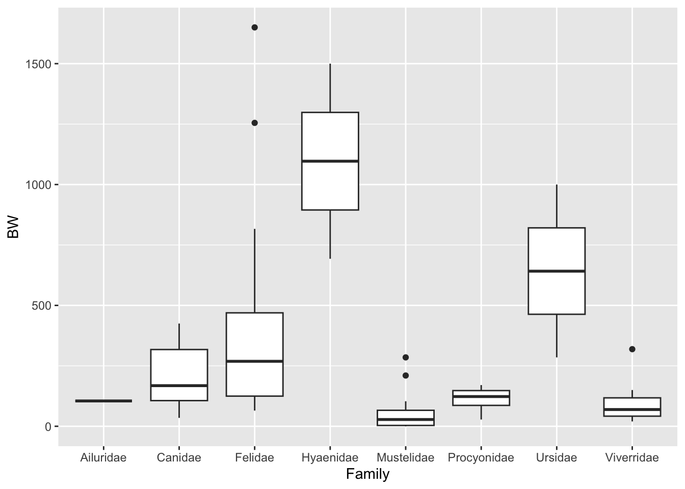
  5. Consider again the carnivora dataset, where BW represents birth weight in grams. Based on the following code, answer the questions below.

    ggplot(carnivora, aes(Family, BW)) + geom_boxplot()
    Warning: Removed 50 rows containing non-finite outside the scale range
    (`stat_boxplot()`).

    fit <- lm(BW ~ Family, data = carnivora)
    anova(fit)
    Analysis of Variance Table
    
    Response: BW
              Df  Sum Sq Mean Sq F value    Pr(>F)    
    Family     7 3256952  465279   6.142 2.648e-05 ***
    Residuals 54 4090670   75753                      
    ---
    Signif. codes:  0 '***' 0.001 '**' 0.01 '*' 0.05 '.' 0.1 ' ' 1
    TukeyHSD(aov(fit))
      Tukey multiple comparisons of means
        95% family-wise confidence level
    
    Fit: aov(formula = fit)
    
    $Family
                                  diff         lwr        upr     p adj
    Canidae-Ailuridae        101.68182  -804.63402 1007.99765 0.9999624
    Felidae-Ailuridae        313.26250  -581.17450 1207.69950 0.9531564
    Hyaenidae-Ailuridae      991.70000   -71.04952 2054.44952 0.0839689
    Mustelidae-Ailuridae     -47.33933  -943.52842  848.84975 0.9999998
    Procyonidae-Ailuridae      6.30000  -963.85314  976.45314 1.0000000
    Ursidae-Ailuridae        537.40000  -464.56985 1539.36985 0.6928677
    Viverridae-Ailuridae      -8.20000  -918.28431  901.88431 1.0000000
    Felidae-Canidae          211.58068  -128.28776  551.44912 0.5157207
    Hyaenidae-Canidae        890.01818   222.98779 1557.04857 0.0023455
    Mustelidae-Canidae      -149.02115  -493.47417  195.43186 0.8692106
    Procyonidae-Canidae      -95.38182  -602.02777  411.26413 0.9988257
    Ursidae-Canidae          435.71818  -129.46904 1000.90540 0.2480542
    Viverridae-Canidae      -109.88182  -489.02093  269.25730 0.9834466
    Hyaenidae-Felidae        678.43750    27.63899 1329.23601 0.0352976
    Mustelidae-Felidae      -360.60183  -672.46244  -48.74123 0.0130218
    Procyonidae-Felidae     -306.96250  -792.03907  178.11407 0.4946297
    Ursidae-Felidae          224.13750  -321.79817  770.07317 0.8970179
    Viverridae-Felidae      -321.46250  -671.25619   28.33119 0.0932343
    Mustelidae-Hyaenidae   -1039.03933 -1692.24376 -385.83491 0.0001564
    Procyonidae-Hyaenidae   -985.40000 -1736.87739 -233.92261 0.0029540
    Ursidae-Hyaenidae       -454.30000 -1246.42672  337.82672 0.6174485
    Viverridae-Hyaenidae    -999.90000 -1672.04181 -327.75819 0.0004772
    Procyonidae-Mustelidae    53.63933  -434.66037  541.93904 0.9999674
    Ursidae-Mustelidae       584.73933    35.93784 1133.54082 0.0290616
    Viverridae-Mustelidae     39.13933  -315.11051  393.38917 0.9999661
    Ursidae-Procyonidae      531.10000  -131.64076 1193.84076 0.2066827
    Viverridae-Procyonidae   -14.50000  -527.85679  498.85679 1.0000000
    Viverridae-Ursidae      -545.60000 -1116.81070   25.61070 0.0710874
    1. Is the group degrees of freedom correct? Explain.

    2. What is the appropriate statistical conclusion from this test?

    3. Write an interpretation of the conclusion with minimal statistical jargon.

    4. Explain why it is appropriate to use Tukey’s HSD here.

    5. What does Tukey’s HSD tell you about these possums?