Logistic Regression

library(ggplot2)
suppressMessages(library(dplyr))
# normal link: elmhurst -> hospital
hospital <- read.csv("https://raw.githubusercontent.com/roualdes/data/refs/heads/master/hospital.csv")

Linear Regression

ggplot(hospital, aes(stay, infection_risk)) +
  geom_point() +
  geom_smooth(method = "lm", se = FALSE)

`geom_smooth()` using formula = 'y ~ x'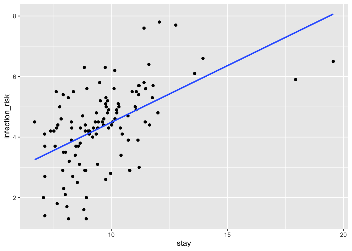

fit <- lm(infection_risk ~ nurses + stay, data = hospital)
summary(fit)

Call:
lm(formula = infection_risk ~ nurses + stay, data = hospital)

Residuals:
     Min       1Q   Median       3Q      Max 
-2.45572 -0.82949  0.06932  0.66121  2.90277 

Coefficients:
             Estimate Std. Error t value Pr(>|t|)    
(Intercept) 0.8970137  0.5387271   1.665  0.09875 .  
nurses      0.0023132  0.0007958   2.907  0.00442 ** 
stay        0.3168527  0.0579818   5.465 2.92e-07 ***
---
Signif. codes:  0 '***' 0.001 '**' 0.01 '*' 0.05 '.' 0.1 ' ' 1

Residual standard error: 1.103 on 110 degrees of freedom
Multiple R-squared:  0.3356,    Adjusted R-squared:  0.3235 
F-statistic: 27.78 on 2 and 110 DF,  p-value: 1.713e-10

df <- data.frame(
  yhat = fitted(fit),
  r = rstandard(fit)
)

ggplot(df, aes(yhat, r)) +
  geom_point()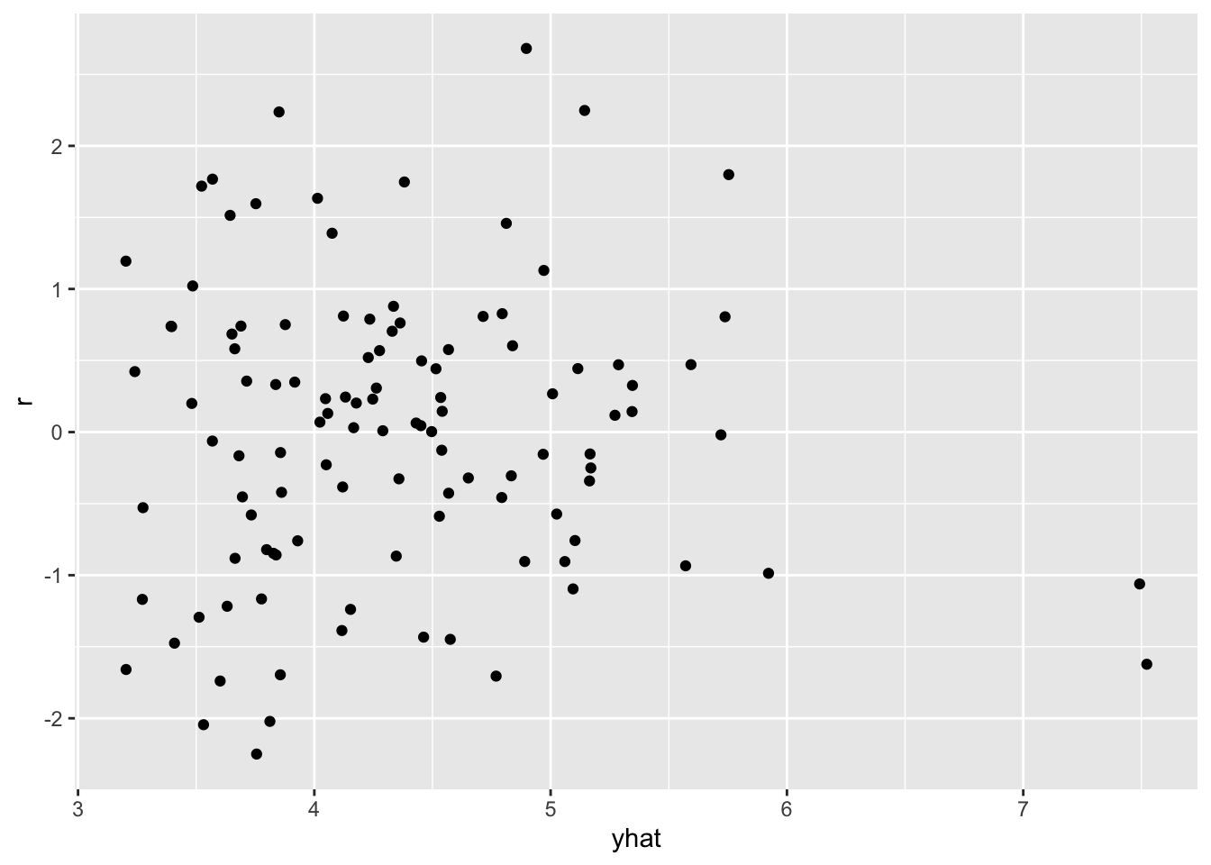

ggplot(df, aes(r)) +
  geom_histogram(bins = 9)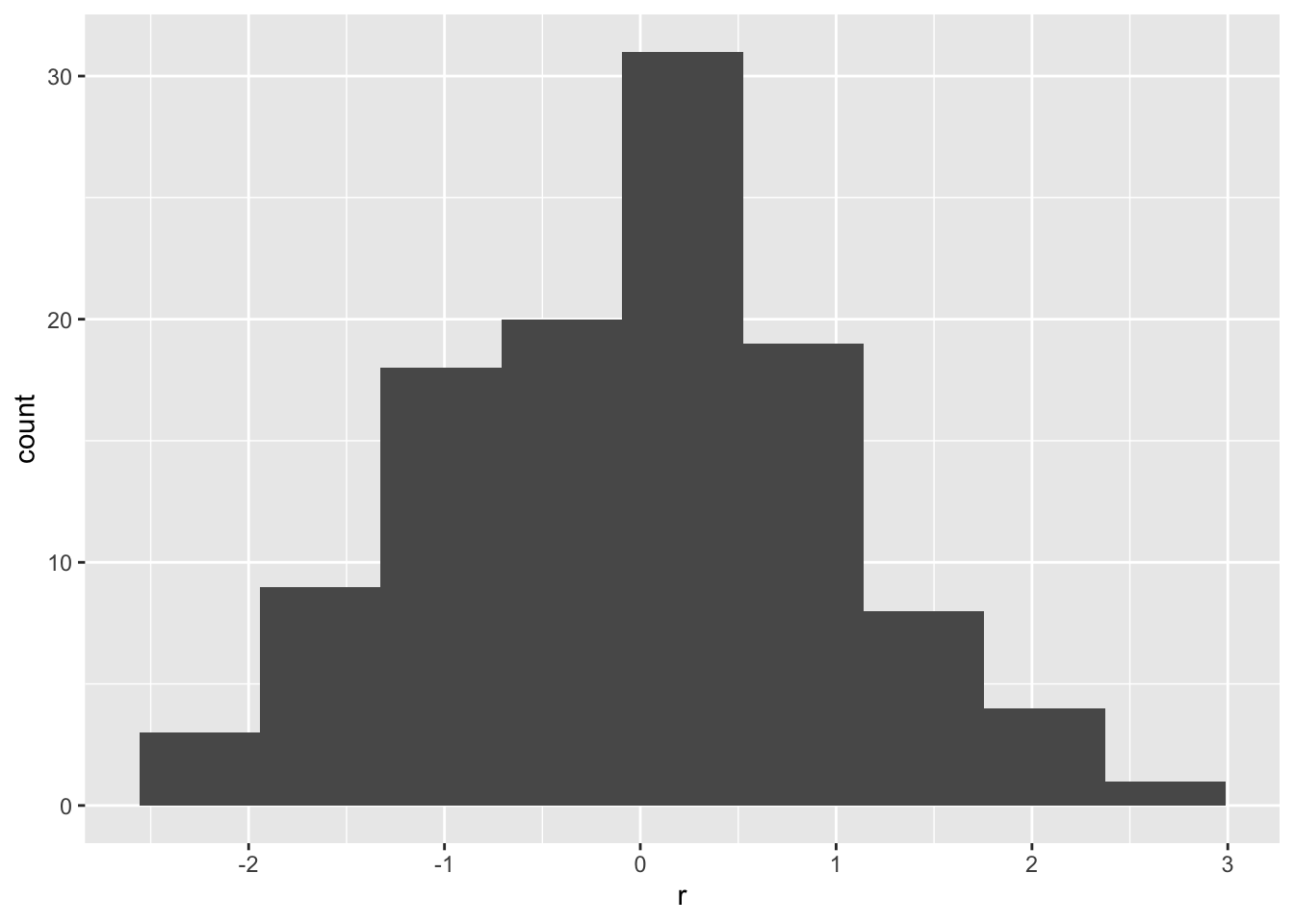

When the number of nurses is fixed at 50, we expect a one day increase in the number of days stayed in a hospital to increase the infection risk by 0.317.

fit %>%
  predict(newdata = data.frame(stay = c(10, 11),
                               nurses = c(50, 50))) %>%
  diff

        2 
0.3168527 

When the number of days in a hospital is fixed at 11, we expect each next nurse to increase the infection risk by 0.002.

fit %>%
  predict(newdata = data.frame(stay = c(11, 11),
                               nurses = c(50, 51))) %>%
  diff

          2 
0.002313205 

Logistic Regression

## normal link: hospital -> possum
possum <- read.csv("https://raw.githubusercontent.com/roualdes/data/refs/heads/master/possum.csv")

ggplot(possum, aes(tailL, pop)) +
  geom_point()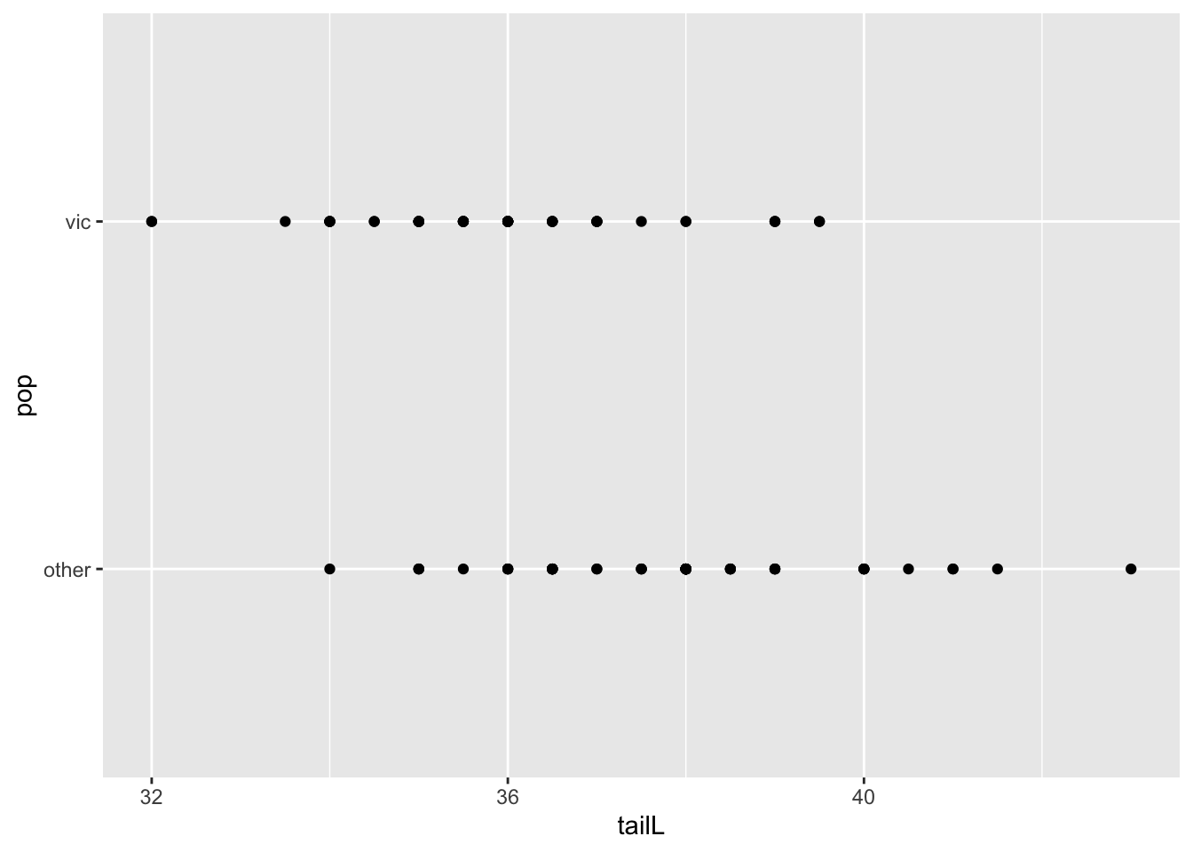

possum <- possum %>%
  mutate(vic = as.numeric(pop == "vic"))

fitl <- glm(vic ~ tailL, data = possum, family = binomial())
summary(fitl)

Call:
glm(formula = vic ~ tailL, family = binomial(), data = possum)

Coefficients:
            Estimate Std. Error z value Pr(>|z|)    
(Intercept)  25.5662     5.8136   4.398 1.09e-05 ***
tailL        -0.6996     0.1580  -4.429 9.45e-06 ***
---
Signif. codes:  0 '***' 0.001 '**' 0.01 '*' 0.05 '.' 0.1 ' ' 1

(Dispersion parameter for binomial family taken to be 1)

    Null deviance: 142.79  on 103  degrees of freedom
Residual deviance: 113.44  on 102  degrees of freedom
AIC: 117.44

Number of Fisher Scoring iterations: 4

o <- order(possum$tailL)
df <- data.frame(
  tailL = possum$tailL[o],
  yhat = fitted(fitl, type = "response")[o]
)

ggplot() +
  geom_point(data = possum, aes(tailL, vic)) +
  geom_line(data = df, aes(tailL, yhat))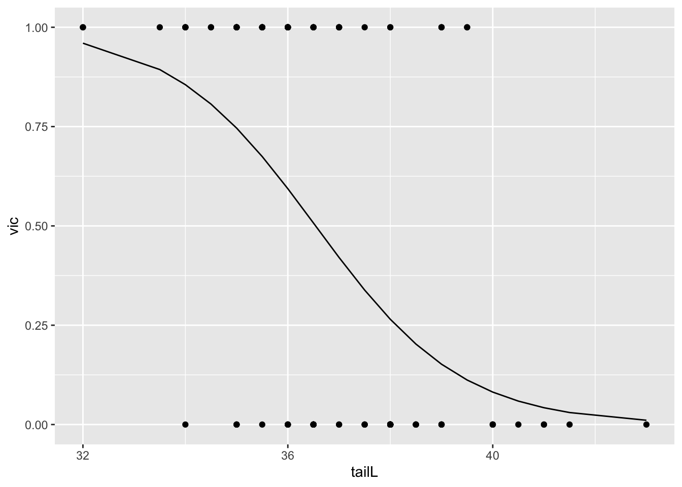

When tail length increases by 1 cm, from 32 to 33 centimeters, we expect the probability that a possum is from “vic” to go down by 0.04.

fitl %>%
  predict(newdata = data.frame(tailL = c(32, 33)), type = "response") %>%
  diff

          2 
-0.03739693 

When tail length is increased by 1 cm, from 42 to 43 centimeters, we expect that probability that a possum is from “vic” to go down by 0.01.

fitl %>%
  predict(newdata = data.frame(tailL = c(42, 43)), type = "response") %>%
  diff

          2 
-0.01069516