Multiple Linear Regression

library(ggplot2)
suppressMessages(library(dplyr))

data(mtcars)

linear regression is linear in a special way

In linear regression, we mean linear in the coefficients. So transformations on \(y\) or \(x\) are encouraged.

ggplot(mtcars, aes(wt, mpg)) +
  geom_point() + 
  geom_smooth(method = "lm", formula = y ~ poly(x, 2),
              se = FALSE)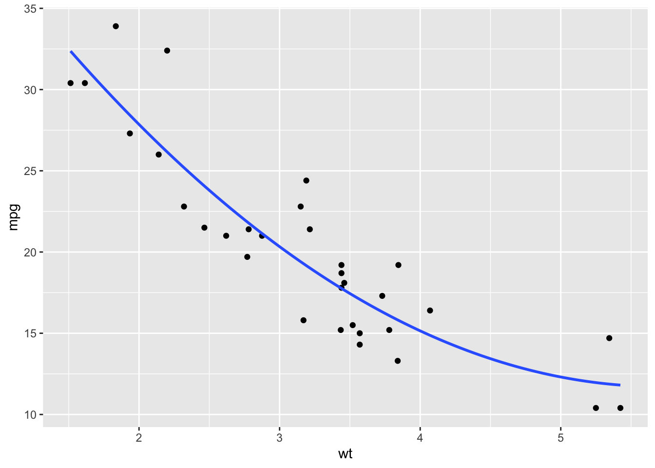

fit <- lm(mpg ~ poly(wt, 2), data = mtcars)

fit <- lm(log10(mpg) ~ log10(wt), data = mtcars)

o <- order(mtcars$wt)
yhat <- 10 ^ predict(fit, newdata = data.frame(wt = mtcars$wt[o]))
df <- data.frame(yhat = yhat, wt = mtcars$wt[o])

ggplot() +
  geom_point(data = mtcars, aes(wt, mpg)) +
  geom_line(data = df, aes(wt, yhat))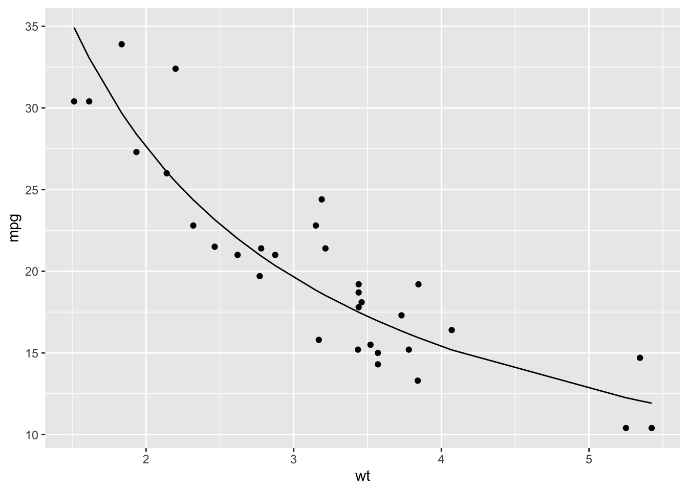

linear regression with multiple numeric explanatory variables

fit <- lm(mpg ~ wt + disp + hp, data = mtcars)
summary(fit)

Call:
lm(formula = mpg ~ wt + disp + hp, data = mtcars)

Residuals:
   Min     1Q Median     3Q    Max 
-3.891 -1.640 -0.172  1.061  5.861 

Coefficients:
             Estimate Std. Error t value Pr(>|t|)    
(Intercept) 37.105505   2.110815  17.579  < 2e-16 ***
wt          -3.800891   1.066191  -3.565  0.00133 ** 
disp        -0.000937   0.010350  -0.091  0.92851    
hp          -0.031157   0.011436  -2.724  0.01097 *  
---
Signif. codes:  0 '***' 0.001 '**' 0.01 '*' 0.05 '.' 0.1 ' ' 1

Residual standard error: 2.639 on 28 degrees of freedom
Multiple R-squared:  0.8268,    Adjusted R-squared:  0.8083 
F-statistic: 44.57 on 3 and 28 DF,  p-value: 8.65e-11

predict(fit, newdata = data.frame(wt = 4, disp = 160, hp = 93))

       1 
18.85446 

confint(fit)

                  2.5 %       97.5 %
(Intercept) 32.78169625 41.429314293
wt          -5.98488310 -1.616898063
disp        -0.02213750  0.020263482
hp          -0.05458171 -0.007731388