Quiz 02

library(ggplot2)
suppressMessages(library(dplyr))
df <- read.csv("https://raw.githubusercontent.com/roualdes/data/refs/heads/master/penguins.csv")

Consider this data set about penguins. We’ll use the variables species, bill_length_mm, and body_mass_g. The bill lengths are measured in millimeters and body mass is measured in grams.

ggplot(data = df, aes(species, bill_length_mm)) +
  geom_boxplot() +
  labs(x = "Species", y = "Bill length (mm)")

Warning: Removed 2 rows containing non-finite outside the scale range
(`stat_boxplot()`).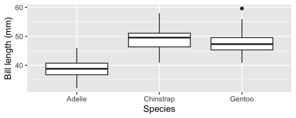

fit <- lm(bill_length_mm ~ species, data = df)
anova(fit)

Analysis of Variance Table

Response: bill_length_mm
           Df Sum Sq Mean Sq F value    Pr(>F)    
species     2 7194.3  3597.2   410.6 < 2.2e-16 ***
Residuals 339 2969.9     8.8                      
---
Signif. codes:  0 '***' 0.001 '**' 0.01 '*' 0.05 '.' 0.1 ' ' 1

1. Write appropriately matching hypotheses for the model (and plot) above.

2. Use the output above to conclude the hypothesis test. Justify your conclusion, citing a p-value.

3. What does your conclusion mean in English?

summary(fit)

Call:
lm(formula = bill_length_mm ~ species, data = df)

Residuals:
    Min      1Q  Median      3Q     Max 
-7.9338 -2.2049  0.0086  2.0662 12.0951 

Coefficients:
                 Estimate Std. Error t value Pr(>|t|)    
(Intercept)       38.7914     0.2409  161.05   <2e-16 ***
speciesChinstrap  10.0424     0.4323   23.23   <2e-16 ***
speciesGentoo      8.7135     0.3595   24.24   <2e-16 ***
---
Signif. codes:  0 '***' 0.001 '**' 0.01 '*' 0.05 '.' 0.1 ' ' 1

Residual standard error: 2.96 on 339 degrees of freedom
  (2 observations deleted due to missingness)
Multiple R-squared:  0.7078,    Adjusted R-squared:  0.7061 
F-statistic: 410.6 on 2 and 339 DF,  p-value: < 2.2e-16

4. Use the output above to calculate and interpret, in context of the data, an intercept for the Species Chinstrap.

ggplot(data = df, aes(bill_length_mm, body_mass_g)) + 
  geom_point() +
  labs(x = "Bill length (mm)", y = "Body mass (g)")

Warning: Removed 2 rows containing missing values or values outside the scale range
(`geom_point()`).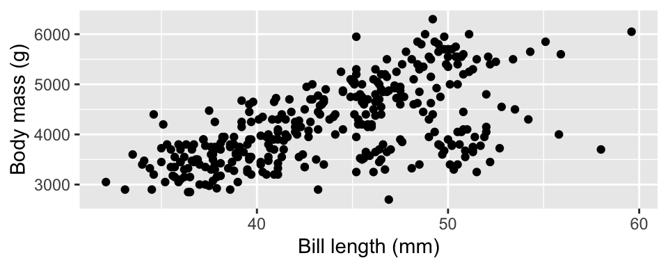

fit <- lm(body_mass_g ~ bill_length_mm, data = df)
summary(fit)

Call:
lm(formula = body_mass_g ~ bill_length_mm, data = df)

Residuals:
     Min       1Q   Median       3Q      Max 
-1762.08  -446.98    32.59   462.31  1636.86 

Coefficients:
               Estimate Std. Error t value Pr(>|t|)    
(Intercept)     362.307    283.345   1.279    0.202    
bill_length_mm   87.415      6.402  13.654   <2e-16 ***
---
Signif. codes:  0 '***' 0.001 '**' 0.01 '*' 0.05 '.' 0.1 ' ' 1

Residual standard error: 645.4 on 340 degrees of freedom
  (2 observations deleted due to missingness)
Multiple R-squared:  0.3542,    Adjusted R-squared:  0.3523 
F-statistic: 186.4 on 1 and 340 DF,  p-value: < 2.2e-16

5. Write appropriately matching hypotheses for the intercept for the model (and plot) above.

6. Use the output above to conclude the hypothesis test. Justify your conclusion, citing a p-value.

7. Interpret the intercept in context of the data.

8. Interpret the slope in context of the data.

9. What units does the slope have?

confint(fit)

                    2.5 %   97.5 %
(Intercept)    -195.02364 919.6371
bill_length_mm   74.82279 100.0078

10. Use the output above to interpret a confidence interval for a term of your choice in context of the data.

predict(fit, newdata = data.frame(bill_length_mm = c(40, 10)))

       1        2 
3858.918 1236.459 

11. Interpret a prediction in context of the data.

12. One of the two predictions is generally considered unreasonable. Which and why?