MATH 314 Exam 02

Exam 02 will take place during the week of May 5 - 8, during our regular class hours and in our regular classroom. Please schedule your preferred time from this Google spreadsheet. You forfeit your right to take Exam 02 by moving someone else's name on this spreadsheeet.

For Exam 02, I need to give you some starter code. This repository will contain the appropriate starter code for your Exam 02. https://classroom.github.com/a/R3YDXhiI

Please clone now this repository to your local machine, so that you can git pull your starter code right before taking Exam 02.

Only these imports are allowed on Exam 02.

import matplotlib.pyplot as plt
import numpy as np
import pandas as pd
import patsy as pt
from scipy.optimize import minimize

Here's some functions you can use during Exam 02.

def lm(theta, X):
	return X @ theta

def mse(y, yhat):
	d = y - yhat
	return np.mean(d * d)

def normal_ll(theta, data):
	y = data['y']
	X = data['X']
	yhat = lm(theta, X)
	return mse(y, yhat)

def windows(N, K):
	w = N // K
	ws = []
	for k in range(K):
		start = k * w
		end = (k + 1) * w
		if k == K - 1:
			end = N
		ws.append((start, end))
	return ws

In general, we should prefer models that predict better on data the model has never seen / been trained on. A common way to measure such prediction accuracy, when one only has one dataset, is to perform $K$ $K$ -fold cross validation. If $K=5$ $K = 5$ , then we will randomly split the dataset up into $5$ $5$ (roughly equal) folds. Then, cycling across all folds, train the model on $4$ $4$ out of $5$ $5$ folds, and measure prediction accuracy on the last (test) fold. Whichever model has lower average (across all test folds) prediction error is considered better.

Use the hospital dataset and $K$ $K$ -fold cross validation to determine which model is a better predictor of infection_risk. Consider a model that uses stay versus a model that uses stay and stay ** 2. Use $K=5$ $K = 5$ . Here's some starter code:
```
...

rng = np.random.default_rng()
N = ...
idx = rng.permutation(np.arange(N))

K = 5
mses = np.zeros(K)
mse2s = np.zeros(K)
ws = windows(N, K)

for k in range(K):
	b, e = ws[k]
	jdx = idx[b:e] # test indices 
	ndx = np.setdiff1d(idx, jdx) # train indices 

	...

(np.mean(mses), np.mean(mse2s))
```
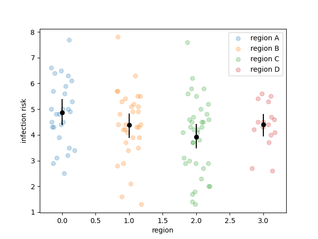
Write a class named LinearRegression that implements the following API
```
lr = LinearRegression('infection_risk ~ stay', df)
lr.fit()
betas = lr.bootstrap()

plt.scatter(betas[:, 0], betas[:, 1]);
```
Your code should work for the example above. Further, for full credit, I will test your code during the exam with a simple change to the code above. Here's the structure of the class I recommend
```
class LinearRegression():
	def __init__(self, ptsystr, df):
		...
	def _lm(self, theta, X):
		...
	def _mse(self, y, yhat):
		...
	def fit(self, y = None, X = None):
		...
	def bootstrap(self, R = 1_000):
		...
```
During Exam 02, I'll ask you to recreate just one of the methods from the above class, and I'll supply the code for the other methods.
Recreate the following plot. The black lines are bootstrapped $95\%$ $95%$ confidence intervals and the black dots are medians ( $50\%$ $50%$ quantiles) which are also calculated from the bootstrap resampled coefficients. There are three distinct steps to recreate this plot:
1. Bootstrap the appropriate model
2. Calculate confidence intervals from the $R$ estimates of the bootstrapped coefficients $\beta$
3. make the plot -- hint: learn that you can loop over the output of df.groupby(...)
During Exam 02, I'll ask you to recreate just one of these parts, and I'll supply the code for the other parts.
The Rayleigh distribution has density function $f(x | \sigma) = \frac{x}{\sigma^2}e^{-x^2 / (2\sigma^2)}$ for $\sigma > 0$ . Use the following $21$ data to find the maximum likelihood estimator of $\sigma$ and to produce a $95\%$ confidence interval using the bootstrap method. [2.55949718, 4.52940383, 3.97518473, 3.38191934, 1.40503558, 1.52411053, 6.91676848, 1.45665845, 2.3602429 , 1.60873959, 3.94374552, 6.22249149, 1.89894113, 5.20759437, 7.24625107, 2.80471966, 4.81060617, 3.08315807, 4.72002917, 1.2751267 , 6.66914935]
Show, empirically (with code), that the procedure to create a $95\%$ $95%$ confidence interval does indeed capture the expectation value in roughly $95\%$ $95%$ of confidence intervals. Your code should repeat the following $R = 1\_000$ $R = 1_000$ times
1. generate $N = 501$ data from the exponential distribution with rate parameter $\lambda = 1$
2. calculate confidence interval (not bootstrap)
3. determine if the confidence interval captures the expectation, call this value c
4. increment a running mean with c using the method defined in Homework 03